TRANSMISSION // 2611.10581v1
Teaching Wireless Models to See Signals at Receiver Resolution
Source published
A preprint introduces a simulated wireless benchmark and a coarse-to-fine generator that improves beam selection and dispersion estimates under a matched network-evaluation budget—not equal computational cost.
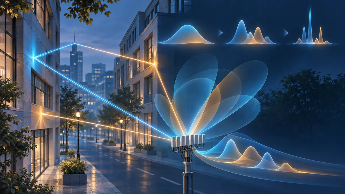
A wireless receiver needs more than a prediction of signal strength. It also matters where the energy arrives from and how long reflected copies take to reach the antenna. A new study asks whether machine-learning benchmarks should represent those signals as a receiver would resolve them, rather than as an idealized list of propagation paths.
From simulated paths to observable signals
Buildings create multiple routes between a transmitter and receiver. A ray-tracing simulator can describe those routes individually, recording their strength, arrival angle and delay. Real receivers, however, have limited resolution: antenna-array size constrains how finely they distinguish directions, while bandwidth constrains how finely they distinguish arrival times.
The study introduces UrbanADPSMap to make those limits explicit. Its two learning targets are the angle power spectrum, or APS, which describes power across arrival directions, and the power delay profile, or PDP, which describes power across arrival times. These quantities support beam selection and help characterize the spread of delayed signal copies.
The benchmark’s central contribution is a shared recipe for converting simulated paths into these spectra. Without that recipe, researchers can start with identical paths yet obtain different targets through different reconstruction choices.
Building a common benchmark
The authors spread each simulated path’s power over angle and delay using mathematical response functions representing finite antenna aperture and bandwidth. They sum those contributions into an angle-delay power map, then sum along its axes to obtain the APS and PDP.
For the reported experiments, the assumed receiver operates at 2.4 GHz with 200 MHz bandwidth and a 16-element uniform linear antenna array. The targets use 180 angular bins and 128 delay bins spanning 0–1,000 nanoseconds. The spectra are packed into a common two-channel format; a validity mask prevents padding from contributing to training losses or evaluation.
UrbanADPSMap contains 2.5 million simulated transmitter–receiver links across 50 urban scenes. Forty scenes supply training data, five validation data and five test data. Keeping each scene entirely within one split tests performance on layouts absent from training, rather than merely on new links in familiar layouts.
Generating a rough sketch, then details
The proposed model, SpecFlowAR, receives an occupancy map and representations of the transmitter and receiver locations. It generates spectra through four resolutions, starting with broad structure and progressing toward sharper peaks and weaker tails.
At the first scale, generation starts from Gaussian noise and uses the scene information alone: there is no previous-scale spectrum. Only subsequent scales use an upsampled output from the preceding scale as a scaffold, alongside the scene information.
The underlying technique is flow matching. During training, the network learns a direction of movement along a path connecting random noise to a target spectrum. During generation, a numerical solver repeatedly evaluates that learned direction to transform noise into a spectrum.
The default setting uses 20 evaluations at each of four scales, totaling 80 network evaluations. Competing iterative generators also receive 80 evaluations. This is a matched network-evaluation budget, not matched computational cost: an evaluation’s expense depends on the architecture and grid resolution.
What improved—and what did not
The main beam-selection measure, BPL@5, asks how much power is lost when choosing the best true beam among five candidates nominated by the predicted spectrum, compared with the best beam overall. Lower values are better.
At 80 evaluations, SpecFlowAR reports 2.03 dB, compared with 2.42 dB for single-scale flow matching and 6.23 dB for the diffusion Transformer baseline. Its reported absolute errors in delay spread and angular spread are also lower: 29.12 nanoseconds and 10.82 degrees, respectively, versus 29.76 nanoseconds and 11.87 degrees for single-scale flow matching.
However, SpecFlowAR does not win every measure. Single-scale flow matching has lower pointwise APS error. That distinction matters: matching every spectrum bin closely and selecting useful beams are related but different objectives.
More evaluations do not consistently improve results either. At the smallest tested budget, 12 evaluations, single-scale flow matching has slightly better beam-selection performance. The study therefore supports metric-specific tradeoffs, not a simple claim that longer sampling always helps.
Limits of the evidence
These are simulated-channel results under a fixed receiver configuration, not a demonstration on measured wireless links. The authors identify measurement-based calibration and variable hardware settings as future work. Reported scene-level confidence intervals overlap for several comparisons, and only five scenes form the test split.
Timing is also setup-specific. Reported APS inference takes 88 milliseconds for SpecFlowAR, 116 milliseconds for single-scale flow matching and 80 milliseconds for the diffusion baseline on an NVIDIA H100. These measurements exclude data loading and transfers; they do not establish a general speed ranking among model families.
The supplied source is the full text of the November 2026 arXiv preprint, not just its abstract. Its findings should be read as preliminary research claims, rather than established deployment evidence.
- wireless channels
- receiver resolution
- angle power spectrum
- power delay profile
- UrbanADPSMap
- SpecFlowAR
- flow matching
- beam selection
- ray tracing
Related reading
Automatically matched by shared topic keywords. These links do not imply that the sources agree or establish a consensus.
Can Wi-Fi predict when its channel needs measuring again?
Source published
Shared keywords: ray tracing
A discrete-time bridge between deterministic diffusion and flow matching
Source published
Shared keywords: flow matching
Keeping Generated Graphs Within Mathematical Bounds
Source published
Shared keywords: flow matching
ChainFlow drafts several AI tokens by predicting where a model’s internal states go next
Source published
Shared keywords: flow matching
Teaching graph generators which hidden dimensions matter
Source published
Shared keywords: flow matching