TRANSMISSION // 2611.05510v1
A faster way to tell faint cosmic signals from photon noise
Source published
Maayane T. Soumagnac and colleagues derive a way to calculate how often random photon counts can mimic a signal after linear filtering. Their numerical methods can replace costly background simulations, although precision limits and the distinction between local and whole-search false alarms remain important.
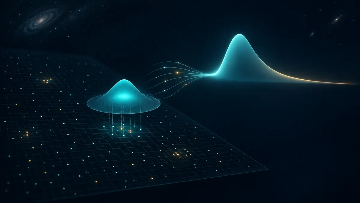
A faint spot in an astronomical image can be a real source—or a chance arrangement of background photons. A new methods preprint turns the calculation of that chance into a deterministic numerical problem, drawing on mathematics also used to model insurance losses.
Detecting a faint astronomical source requires more than finding a bright-looking patch. Astronomers also need to know how often background noise alone would produce a detection statistic at least as large. That probability helps set the threshold for declaring a detection.
In Fast and accurate false-alarm probabilities for linear detection statistics in Poisson noise, Maayane T. Soumagnac, Eran O. Ofek, Shachar Israeli and David Glukhov derive a faster way to calculate this probability. Their work is a mathematical and computational study, not a report of a newly observed celestial object. Version 1 was submitted to arXiv on November 3, 2026; its landing page says “Submitted to ApJS,” which does not establish acceptance or completed peer review.
Why sparse photons complicate detection
In low-count images, background fluctuations follow Poisson statistics. The paper highlights X-ray astronomy, while also noting relevance to ultraviolet, gamma-ray and neutrino measurements. In this regime, a Gaussian approximation is no longer adequate for the detection problem described by the authors.
A common detection statistic is a weighted sum of measurements in nearby pixels. The weights form a filter, which can use information about the expected shape of a source. Simply adding counts inside a box preserves a straightforward Poisson distribution, but applying different weights generally produces a more complicated distribution.
One way to find the corresponding detection threshold is to simulate many background-only images, filter each one and count how frequently large values occur. Rare false alarms make this expensive. For a false-alarm probability of one in ten million, about ten million independent realizations are needed just to expect one event in the relevant tail—not to measure its probability precisely.
Count contributions, not image configurations
The authors’ central step is to describe the filtered background through individual photons rather than through all possible arrangements of pixel counts.
Each background photon contributes the filter weight at the pixel where it lands. The detection statistic is the sum of those contributions. Because the total number of background photons is itself Poisson distributed, this sum is a compound Poisson random variable: a random number of random contributions added together.
For a uniform background, the distribution of a single photon’s contribution is simply a normalized histogram of the filter weights. For a spatially varying background, the histogram is weighted by the expected background counts in each pixel. Together with the expected total photon count within the filter’s support, this determines the background-only distribution of the statistic.
Compound distributions are already well studied, including in insurance risk calculations. The paper also acknowledges related astronomical work. Its specific construction treats the photons themselves as the events contributing to a linear detection statistic.
Two numerical routes
The researchers implement two ways to calculate the resulting distribution. One uses the Fast Fourier Transform, or FFT, to replace repeated convolutions with efficient operations in Fourier space. The other uses Panjer recursion, building each probability from previously calculated probabilities.
These approaches have different practical limits. The FFT implementation can handle filters containing negative weights, but extremely small probabilities can lose accuracy when Fourier contributions nearly cancel. The paper illustrates resulting oscillations in the distribution’s far tail.
Panjer recursion avoids that cancellation mechanism. However, the implementation presented requires non-negative discretized filter weights. A filter with negative regions, such as a Mexican-hat wavelet, therefore needs another implementation, such as the FFT approach.
For the illustrated five-by-five-pixel filter, the paper reports an FFT calculation taking about 30 milliseconds, compared with roughly 10–12 seconds for simulations. The four compared methods produced detection thresholds differing by about one percent. These are results for the reported example, not a universal speed guarantee.
What the calculation does—and does not—establish
The mathematical formulation assumes independent Poisson background counts and specified expected background levels. Its numerical implementations also discretize filter weights and limit the computational range. The authors check stability by refining the discretization and tightening bounds on omitted probability. Thus, an exact distributional formulation does not mean unlimited numerical precision.
Crucially, the calculation gives a local false-alarm probability, not the probability of obtaining a false detection somewhere across an entire search. The authors explicitly leave the look-elsewhere effect outside their calculation; a global assessment requires that additional accounting.
Within those boundaries, the contribution is practical: calculating detection significance need not always depend on accumulating enormous simulated samples. The authors describe open-source Python and MATLAB implementations intended to make the method usable in photon-counting detection problems.
- astrophysics
- photon counting
- Poisson noise
- false-alarm probability
- source detection
- compound Poisson distribution
- Fast Fourier Transform
- Panjer recursion