TRANSMISSION // 2609.24609v2
GraphToolbox puts electricity-forecasting models on a common track
Source published
An open-source framework makes it easier to compare graph neural networks for electricity forecasting. In tests using French data, graph models performed well on net load—the demand remaining after wind and solar generation are subtracted—while results for ordinary load were more mixed. The study also examines how combining or updating models can affect accuracy.
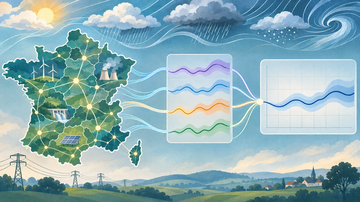
Electricity demand in one region can vary alongside demand in others. Graph neural networks (GNNs) represent these relationships as links, then pass information along them to make forecasts. Comparing GNN designs can be difficult when experiments use different data processing, training choices or evaluation methods. GraphToolbox aims to make comparisons easier by bringing these steps into a shared framework.
The challenge of a fair comparison
A GNN forecaster has several moving parts: how its graph is built, which operation passes information between connected regions, how the model is trained and how predictions are assessed. Changing several parts at once can make it hard to tell what explains a difference in accuracy.
In this preprint, Eloi Campagne and colleagues introduce GraphToolbox, an open-source Python framework built on PyTorch Geometric. Its configuration-driven pipeline brings graph construction, training, model comparison, forecast combination and interpretation into one workflow. The researchers report that it can run 53 of the 65 graph-convolution operators they tested without modifying those operators. It also includes statistical tests for comparing forecasts and tools for examining feature and edge attributions.
The team used the framework to benchmark French electricity load and net load. Load is electricity demand; net load is demand minus wind and solar generation. They used half-hourly data for 12 French regions from 2015 through 2019, with 2019 as the test year, and assessed the sum of regional forecasts at the national level. For the main comparisons, they generally held the data, split and training setup fixed while changing one modelling choice at a time.
Different targets, different results
For ordinary load, the evaluated graph convolutions generally beat the additive, recurrent and foundation-model references in the reported comparison. But the tests did not establish a clear winner among graph convolutions. Pooled XGBoost—a tree-based method trained on the same inputs as the graph models—had a lower national root mean squared error (RMSE) than the best individual graph model in the main run, though the difference was not statistically significant. The authors also report that the ordering of individual graph architectures was not stable across training seeds.
Two other strategies improved load forecasts in these experiments. An online expert mixture adjusted the weights given to different models based on their recent errors; it performed better than the best individual convolution in the reported test. Daily updates to a graph model also improved its accuracy. These results apply to the methods and test setup studied; they do not show that combining or updating models will help in every forecasting system.
Net load produced a different pattern. The graph models outperformed the additive, recurrent and XGBoost baselines reported for that task. Forecasting load, wind and solar separately and then recombining their predictions improved the graph models further. The authors note a trade-off: this approach uses three models for one forecast, so the comparison is not matched on total training computation.
What the results do—and do not—show
The controlled comparisons help clarify what a benchmark can support. In an identity-graph comparison, which removes message passing between regions while keeping a common model setup, message passing helped most of the tested operators on load. But the authors caution that it explains only part of the overall performance difference: graph models also involve choices such as parameter sharing and multi-step prediction. The result does not establish that adding regional links will always improve forecasts.
The findings also depend on the information supplied to the models. In the benchmark, weather observations from the forecast day were treated as known inputs. The authors say this “perfect-forecast” assumption makes errors lower than those expected in an operational forecast using weather predictions. For net load, the graph model’s advantage over additive references also depended on forecast-day wind and cloud information.
There are further limits. The accuracy benchmark covers two tasks, one territory and one test year, so it cannot establish how well the findings transfer elsewhere or across different conditions. Most architecture comparisons used one training run per model; separate repeated-seed tests show that training variability can affect the fine ordering. The statistical tests account for uncertainty across the test window, not jointly for test-window and retraining variability. The authors also state that their interpretability measures are associational, not evidence that a particular region or graph link causes a forecast change.
GraphToolbox is presented as both software and a way to make controlled forecasting comparisons more practical. The benchmark suggests that model aggregation, adaptation and target definition deserve attention alongside the choice of GNN architecture. These findings come from an arXiv preprint; the available source does not establish its peer-review status.
- electricity forecasting
- graph neural networks
- benchmarking
- net load
- forecast aggregation
- open-source software
Related reading
Automatically matched by shared topic keywords. These links do not imply that the sources agree or establish a consensus.
A Python toolkit for building and testing supply-chain simulations
Source published
Shared keywords: open source software
SIMBAD tests when traffic forecasts should trust the past
Source published
Shared keywords: graph neural networks
A graph-learning method updates its view as connections appear
Source published
Shared keywords: graph neural networks
A New Geometry for Graphs Whose Neighbors Differ
Source published
Shared keywords: graph neural networks
Combining reviews, photos and descriptions helps recommend less-popular products
Source published
Shared keywords: graph neural networks