TRANSMISSION // 2026.11.05.764527v1
Which parts of wheat growth stay consistent across environments?
Source published
A Bayesian model fitted to simulated wheat growth separated genetic, environmental and interaction effects. Growth timing and curve shape showed relatively little genotype-by-environment interaction, while the final biomass level showed much more. Real-world prediction and breeding benefits remain untested.
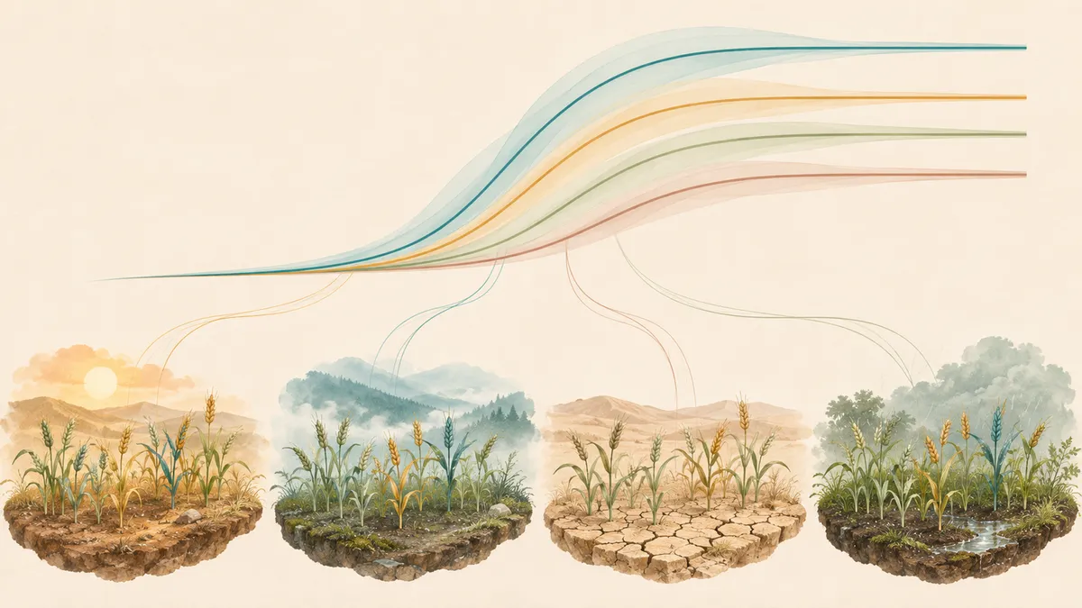
A plant’s growth curve contains more information than its final size. A new simulation study asks which features of that curve might help characterize wheat genotypes across different growing conditions—and which remain strongly dependent on the environment.
Can the way wheat grows reveal something consistent about its genetics, even when growing conditions change? A study first-authored by Shota Gugushvili investigates that question by separating growth curves into interpretable features. Its main finding is a distinction: the timing and shape of simulated biomass growth showed relatively little genotype-by-environment interaction, whereas the eventual biomass level showed considerably more.
The work is a bioRxiv preprint, posted November 6, 2026, and has not been peer reviewed. It analyzes computer-generated wheat data, not newly conducted field trials, and demonstrates neither improved crop yields nor better breeding outcomes.
Turning growth into three features
Repeated observations of plant characteristics are called longitudinal phenotypes. Rather than recording only an end-of-season value, they describe development through time. The authors’ motivation includes drone-based observations, which may provide only around 10–15 measurements during a growing season—too few to support arbitrarily complicated growth models.
The researchers used a smooth, S-shaped log-logistic curve with three adjustable parameters. The upper asymptote is the biomass level the curve approaches as growth levels off. The midpoint is the time at which biomass reaches half that level. The slope parameter controls the curve’s steepness around the midpoint. Biomass here means plant material, not harvested grain yield.
Each parameter was modeled as a combination of an overall baseline, a genotype contribution, an environment contribution and an interaction. A genotype is a plant’s genetic makeup. Genotype-by-environment interaction, often shortened to G × E, means that genetic differences have different effects under different conditions. For example, the biomass advantage of one genotype over another might be larger in one environment than another; their rankings need not reverse for an interaction to occur.
Sharing information without assuming identical plants
Bayesian hierarchical modeling combines two ideas. Bayesian inference updates starting probability distributions, called priors, using the data to obtain updated distributions, called posteriors. A hierarchical model links individual groups through shared distributions. Here, growth curves for different genotypes and environments were fitted together, allowing them to share information without forcing them to be identical.
This sharing can pull poorly supported estimates toward the broader pattern, a process called shrinkage. The framework also carries uncertainty through the analysis instead of treating estimated growth parameters as perfectly known.
Uncertainty means the range of parameter values or observations that remain plausible given the data and modeling assumptions. A 95% Bayesian credible interval describes a range containing 95% of the posterior probability for a parameter. A prediction band instead describes plausible observations at a particular time. Neither guarantees that the model captures all the complexities of real plants.
The demonstration used APSIM-Wheat simulations for 48 genotypes selected from an original panel of 199. Four Australian locations—Emerald, Narrabri, Yanco and Merredin—were represented over 31 growing seasons, giving 124 location-year environments and 5,952 genotype–environment combinations. Biomass values were sampled every two weeks. The first 14 days after sowing were excluded because near-zero values caused numerical fitting problems.
The final biomass level stood apart
The fitted curves closely followed the simulated trajectories, although the smooth model missed small bumps that the authors suggest may reflect short-term weather events. Across all three growth parameters, environmental effects contributed the most variation, followed by genotype effects and then interactions.
The researchers compared interaction standard deviations with genotype standard deviations. The reported ratios were 0.6–0.9 for the upper asymptote, 0.25–0.35 for the midpoint and 0–0.1 for slope. These are comparisons of statistical spread, not percentages of total variation explained.
For the asymptote, 2,173 interaction estimates—36.5% of genotype–environment combinations—had 95% credible intervals excluding zero. The corresponding figures were 91, or 1.5%, for midpoint and none for slope. Intervals containing zero do not prove an interaction is absent, but the overall pattern identifies final biomass as the more environment-dependent genetic feature in this analysis.
The authors also grouped environments into three clusters using estimated environmental effects. These largely tracked location differences. Grouping interactions by these environment types was about as effective as grouping by location, with comparable unexplained interaction remaining.
What remains to be demonstrated
The relatively stable timing and slope parameters could become useful inputs to future prediction models. That possibility is not evidence of successful prediction in unfamiliar fields. Even little interaction at the parameter level does not rule out interaction in the full, nonlinear growth trajectory.
The simulations contained no added measurement noise, unlike real sensor observations. The fitted model assumed independent, normally distributed errors with constant spread, and did not explicitly incorporate changing temperature, sunlight or soil water as growth drivers. Testing real observations, modeling the interaction in final biomass and linking growth features to yield remain necessary steps.
Corteva Agriscience supported part of the research; four authors were Corteva employees when the manuscript was conceived.
- wheat
- Bayesian hierarchical modeling
- genotype-by-environment interaction
- plant growth
- longitudinal phenotypes
- biomass
- APSIM
- uncertainty